Notional DSCOVR Faraday Cup Instrument “Calibration” and Data Analysis Procedure
The following describes a potential new framework for the DSCOVR Faraday Cup (FC) science data analysis pipeline.
DSCOVR Measurement Description
DSCOVR FC data are de-commutated and grouped into measurement spectra/cycles, each comprising signals measured by the A, B, and C sensor segments over an ascending sequence of modulator voltages. The signal and voltage are initially in data number units. The range of possible signal values is 0-3072 and the range of possible voltage values is 0-63. The group of ascending voltages that constitute one spectrum can be anywhere from 19 to 64 measurements long.
For each spectrum, the objective is to derive the solar wind ion density, thermal speed, and velocity vector (n,w,v).
Current pipeline method
At present, the raw data are converted to physics units using a calibration table, summed over the sensor segments, and recast as phase space distribution functions. A variety of ad hoc operations are invoked in order to tweak the background subtraction, isolate the physically relevant sub-range in voltage, and remove transients. Then a Gaussian peak fitting is performed. The parameters of the Gaussian map directly to (n, w, | v |). Finally, the ratios between the signal peak values are fed into a table lookup to estimate the flow angle and complete the velocity vector.
Current issues
The instrument has long experienced grounding faults and possibly other issues that introduce noise, transients, harmonics, and other ugliness into the signal. We have built a manifold of if-then inspections and corrections to try to deal with them, but the complexity and ad hoc nature of it makes validation, revision, and recalibration not only difficult to accomplish but also difficult to define clearly. The pipeline itself is also computationally inefficient.
Potential resources you can leverage
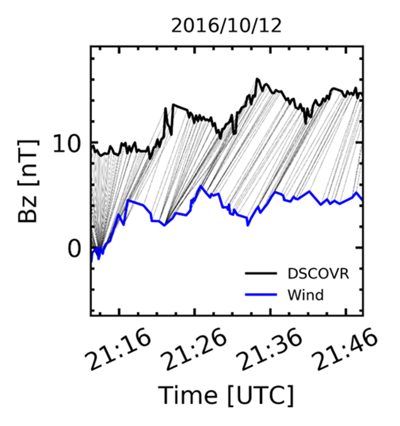
Perhaps the best-calibrated Faraday Cup instrument in space is onboard the Wind spacecraft, which observes continuously and, like DSCOVR, orbits the Earth-Sun L1 point. The vast majority of the time, Wind and DSCOVR are observing very similar or even identical plasmas, offset from one another only a bit in space and time. The DSCOVR experiment, and all solar wind experiments, are calibrated and validated via time-shifted comparisons with Wind. The Faraday Cup instrument onboard the DSCOVR and Wind spacecraft are nearly identical, but with some differences in how they area integrated onto the spacecraft bus related to electrical grounding, which results in the different peak tracking behavior.
A possible approach
Since so much of the instrument behavior is a black box, you could consider modeling it as such. You could attempt to leverage the abundant ground truth from Wind to train a neural network that can perform the required data analysis end to end.
For example, you could take the following steps:
Step One
Collect the Wind and DSCOVR magnetic field data sets, BW(t) and BD(t), for a period of time deemed suitable for training.
- These data are archived at: https://cdaweb.gsfc.nasa.gov/pub/data/wind/mfi/mfi_h2/2022/ And https://cdaweb.gsfc.nasa.gov/pub/data/dscovr/h0/mag/2022/ respectively.
- To obtain data for other years, replace the “2022” in the above URLs with the desired year (e.g., 2021, 2020)
- You may also use the manual interface at https://cdaweb.gsfc.nasa.gov/ and select Wind, Magnetic Fields, H2 data type, and then enter a date range
- The Time Period should be long enough for thorough training, i.e., a fairly complete representation of plasma conditions. This is not going to be unsupervised, so a few months at minimum is suggested for the training period.
- The Time Period otherwise should be as short as possible so as to capture stable instrument performance (the timescale on which incremental instrument degradation becomes noticeable is about a year)
- Attempt some kind of "clean up" where you remove periods containing clear qualitative differences between the two data sets; i.e., structures that are simply not present in both. (Alternatively, you could do this “clean up” in Step Three.)
Step Two
Derive optimal Dynamic Time Warping (DTW) mappings, D(t), between the two data sets (Owens et al example)
- DTW mapping is just a one-to-one lookup. For time t at DSCOVR, the corresponding measurement at Wind occurs at t' = D(t). See the illustrative example below.
- DTW mapping is performed following methodologies of Prchlik et al, Owens et al-- use a preexisting nonlinear optimization algorithm to optimize a correlation measure, Pτ( BW(D(t)), BD(t) ), where the timescale, τ, is on the order of hours to days. The optimization is subject to some sensible constraints, for example:
- Limiting the overall timeshift |t - D(t)|. Given how close the two spacecraft are in space, it wouldn't be physical for one to see a solar wind feature and then the other to see it hours or days later. The characteristic timescale is seconds to minutes.
- Limiting the time distortion dD/dt. For example, a blob that takes 10 minutes to cross DSCOVR ought not cross Wind in 1 second.
Step Three
Select time series from the Wind ion parameters (density, n(D(t)); temperature, w(D(t)); velocity, v(D(t))) for time periods where Pτ( BW(D(t)), BD(t) ) is near unity. This will be the ground truth. You could train the DSCOVR data analysis to produce these parameters.
The Wind ion parameters are archived here: https://cdaweb.gsfc.nasa.gov/pub/data/wind/swe/swe_h1/2022/
- To obtain wind ion parameters for other years, replace the “2022” in the above URL with the desired year (e.g., 2021, 2020)
- You may also use the manual interface at https://cdaweb.gsfc.nasa.gov/ and select Wind, Magnetic Fields, H2 data type, and then enter a date range
Step Four
Prepare representations of the DSCOVR spectra at the corresponding set of time points.
- The DSCOVR data are current vs. voltage spectra, so one time point consists of a series of currents measured at each of ~20 [variable] voltage steps. There are three sectors to the cup, so overall a typical spectrum is like 60 measurements, 20 each from sectors A, B, and C. The set of voltage steps changes from one spectrum to the next; it isn't always the same and it can have anywhere from 19 to 60 steps.
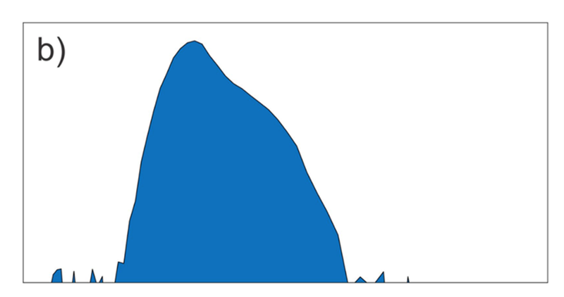
- There may be multiple ways to do this, but one approach is to just plot it up.. Vech et al (2020) literally made standardized jpeg plots of the spectra in physics units and fed them into an image recognition AI, which was expedient. The figure below (figure 1b from his paper) shows an example of current-voltage spectra in the exact format passed to the trained algorithm. There may be something simpler, but the Vech method took advantage of the fact that image recognition is a major machine learning application with tons of user-friendly tools all ready to go.
- The measurements need not be converted to physical units. One can take the raw data numbers from the instrument and flatten/renormalize/offset/otherwise prepare in whatever format interfaces well with the training algorithm of choice. This is the data set.
Step Five
Train a neural network to predict the Wind n(D(t)), w(D(t)), and v(D(t) values from the DSCOVR data.
- The standard protocol in machine learning applications is to now cut the data set into two groups, one of which is training data and the other of which is test data.
- Train a neural network to predict the corresponding ground truth from the training data, and assess performance against the test data ground truth by applying the trained network to the test data. You could use preexisting open-source software for all of this. Refine as necessary.
- Compare neural network prediction accuracy to figures from prior Wind-ACE and Wind-DSCOVR comparisons (we've done some work on this already and have a good idea what kind of differences one should get from "perfectly" calibrated data).
For Steps Four to Five, we have since experimented with SKLEARN and KERAS (from tensorflow). For a basic proof of concept, we used a 3-layer sequential ANN with 30- vector input (simulated data comprising current measurements over 30 voltage windows) and 3-vector output (density, speed, temperature). We used simple chi-sq for the loss function. A hastily trained ANN was good enough to get us in the 10% range for our simulated data. Most importantly, our simulated data was modeled after raw DSCOVR fc data numbers, suggesting this method could be used with the unprocessed, uncalibrated measurement series.
Another option: Valid Data Classifier?
One additional thing that you could do to make this implement smoothly is to train a separate classification AI to recognize useful inputs. DSCOVR measurements are occasionally invalid because of energy tracking errors, oscillations, and/or noisy transients. In those cases, one usually gets bad fits, however what is and isn't a bad fit is not always obvious, particularly from a cursory look at the outputs. Usually, when examining the inputs that produce a bad fit, one can recognize why and how it went wrong. This effort is very time consuming, however, and the variety of failure modes makes catch-all screening very difficult. Perhaps a simpler AI could be trained to recognize this broad range of anomalous inputs.